Week 10: Working with weighted data
PUBPOL 750 Data Analysis for Public Policy I
Justin Savoie
MPP-DS McMaster
2022-07-22
1 / 19
Working with weighted data
2 / 19
Weighted data
- Often the data you will be working with is weighted
- This could, in theory, apply to any type dataset
- Policy cases could be weighted, counties could have weights
- In practice, weighted data is usually data collected on individuals. Intuitively, some individuals are less likely to be represented in your data, they are harder to reach, and you want to increase their weight in your analysis
- Weights allow for a dataset to be corrected so that results more accurately represent the population being studied.
3 / 19
Sampling
- Why can we claim that a poll of 100 respondents represent the views of 38M of Canadians ?
- Random sampling: if we select respondents truly randomly, the results are very close to true population numbers
- Random digit dialing + random selection within the household
- Complex survey designs: strata, clusters
- Complex Surveys: a guide to analysis using R
- Applied Survey Data Analysis
4 / 19
Working with existing weights
- Weights are often calculated by raking: adjusting weights algorithmically to match marginals distributions
- Marginal distributions are simply the general distribution in the population. We call it "marginal" to distinguish them from a "conditional" distribution which are, for example, the distribution of age, given gender or education.
- To calculate weights: you pick which variables you want to weight on. Provide the true numbers in the population for those distribution (marginal distribution). Let R algorithmically create weights. Will provide an example at the end.
5 / 19
Working with existing weights
- Almost all the time, weights either have a mean of 1 or sum to 1. Sometimes weight sum to the population size.
- Weights with a mean of one attribute how much respondent is worth in that sample.
- It's not very important which scale the weights are one (if they sum to 1 or sum to the sample size or the population). You can always scale them back (if the weights sum to 1, multiplying them by N has them average to 1, multiplying them by the population has them sum to the population, and vice versa).
- Importantly, it will not affect your analyses.
6 / 19
Simple weighted mean
library(tidyverse)library(readstata13)library(survey)df <- read.dta13("~/Downloads/2019 Canadian Election Study - Phone Survey v1.0.dta") %>% as_tibble()mean(df$q14)## [1] 46.36732weighted.mean(df$q14,df$weight_CES)## [1] 46.751917 / 19
df %>% group_by(q31) %>% summarise(nweighted=sum(weight_CES),n=n()) %>% ungroup() %>% mutate(wp=nweighted/sum(nweighted),p=n/sum(n))## # A tibble: 5 × 5## q31 nweighted n wp p## <fct> <dbl> <int> <dbl> <dbl>## 1 (-9) Don't know 113. 117 0.0282 0.0291 ## 2 (-8) Refused 8.22 7 0.00204 0.00174## 3 (1) Better 853. 818 0.212 0.203 ## 4 (2) Worse 1270. 1316 0.316 0.327 ## 5 (3) About the same 1776. 1763 0.442 0.4388 / 19
CESDesign <- svydesign(ids = ~0, weights = ~weight_CES, data = df)svymean(~q14, CESDesign)## mean SE## q14 46.752 0.5594q14mean <- svymean(~q14, CESDesign)confint(q14mean)## 2.5 % 97.5 %## q14 45.65546 47.84836t.test(df$q14)[[4]]## [1] 45.44254 47.29210## attr(,"conf.level")## [1] 0.9547.29210-45.4425;47.84836-45.65546## [1] 1.8496## [1] 2.19299 / 19
svytable(~q31, CESDesign)## q31## (-9) Don't know (-8) Refused (-7) Skipped (1) Better ## 113.385743 8.218755 0.000000 852.964985 ## (2) Worse (3) About the same ## 1270.314932 1776.115585svyby(~q31,by=~age_range, CESDesign,svymean)## age_range q31(-9) Don't know q31(-8) Refused## (1) 18-24 years old (1) 18-24 years old 0.09858770 0.003671925## (2) 25-34 years old (2) 25-34 years old 0.05292624 0.003662916## (3) 35-44 years old (3) 35-44 years old 0.03218542 0.001306650## (4) 45-54 years old (4) 45-54 years old 0.01587141 0.000000000## (5) 55+ years old (5) 55+ years old 0.01493389 0.002451560## q31(-7) Skipped q31(1) Better q31(2) Worse## (1) 18-24 years old 0 0.1356857 0.3535161## (2) 25-34 years old 0 0.2031205 0.3338878## (3) 35-44 years old 0 0.1922825 0.3447326## (4) 45-54 years old 0 0.2099687 0.3304475## (5) 55+ years old 0 0.2334403 0.2888716## q31(3) About the same se.q31(-9) Don't know## (1) 18-24 years old 0.4085385 0.021733816## (2) 25-34 years old 0.4064025 0.011124884## (3) 35-44 years old 0.4294928 0.007988759## (4) 45-54 years old 0.4437124 0.005838565## (5) 55+ years old 0.4603027 0.003182128## se.q31(-8) Refused se.q31(-7) Skipped se.q31(1) Better## (1) 18-24 years old 0.003668756 0 0.02578584## (2) 25-34 years old 0.003654493 0 0.02000676## (3) 35-44 years old 0.001306358 0 0.01704271## (4) 45-54 years old 0.000000000 0 0.01774903## (5) 55+ years old 0.001395807 0 0.01192614## se.q31(2) Worse se.q31(3) About the same## (1) 18-24 years old 0.03518463 0.03584606## (2) 25-34 years old 0.02347812 0.02450288## (3) 35-44 years old 0.02076485 0.02173208## (4) 45-54 years old 0.02006696 0.02150164## (5) 55+ years old 0.01248310 0.0139373010 / 19
Making your own weights
df_sub <- df %>% select(q31,q4,q3,age_range) df_sub <- df_sub %>% mutate_all(as.character)marginals <- c(`(Intercept)`= 1, c(#`q4(1) Newfoundland and Labrador` = 0.0115942028985507, `q4(10) British Columbia` = 0.144927536231884, `q4(2) Prince Edward Island` = 0.00289855072463768, `q4(3) Nova Scotia` = 0.0289855072463768, `q4(4) New Brunswick` = 0.0289855072463768, `q4(5) Quebec` = 0.231884057971014, `q4(6) Ontario` = 0.376811594202899, `q4(7) Manitoba` = 0.0289855072463768, `q4(8) Saskatchewan` = 0.0289855072463768, `q4(9) Alberta` = 0.115942028985507),c(#"q3(1) Male"=0.48, "q3(2) Female"=0.48, "q3(3) Other"=0.04),c(#"age_range(1) 18-24 years old"=0.1, "age_range(2) 25-34 years old"=0.2, "age_range(3) 35-44 years old"=0.15, "age_range(4) 45-54 years old"=0.2, "age_range(5) 55+ years old"=0.35))11 / 19
tmp_form <- paste(" ~ 1 + q4 + q3 + age_range")surveyDesign <- svydesign(id = ~ 1, weights = ~ 1, data = df_sub)surveyDesign <- calibrate(design = surveyDesign, formula = as.formula(tmp_form), calfun = "raking", population = marginals, maxit = 2000)df_sub$weight <- weights(surveyDesign)12 / 19
plot(df_sub$weight*nrow(df_sub),df$weight_CES)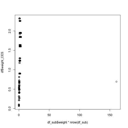
13 / 19
df_sub %>% arrange(desc(weight))## # A tibble: 4,021 × 5## q31 q4 q3 age_range weight## <chr> <chr> <chr> <chr> <dbl>## 1 (3) About the same (10) British Columbia (3) Other (2) 25-34 years … 4.00e-2## 2 (3) About the same (6) Ontario (2) Female (1) 18-24 years … 8.88e-4## 3 (1) Better (6) Ontario (2) Female (1) 18-24 years … 8.88e-4## 4 (2) Worse (6) Ontario (2) Female (1) 18-24 years … 8.88e-4## 5 (1) Better (6) Ontario (2) Female (1) 18-24 years … 8.88e-4## 6 (-9) Don't know (6) Ontario (2) Female (1) 18-24 years … 8.88e-4## 7 (3) About the same (6) Ontario (2) Female (1) 18-24 years … 8.88e-4## 8 (3) About the same (6) Ontario (2) Female (1) 18-24 years … 8.88e-4## 9 (2) Worse (6) Ontario (2) Female (1) 18-24 years … 8.88e-4## 10 (3) About the same (6) Ontario (2) Female (1) 18-24 years … 8.88e-4## # … with 4,011 more rows14 / 19
df_sub$weight[df_sub$weight>quantile(df_sub$weight,0.99)] <- quantile(df_sub$weight,0.99)plot(df_sub$weight*nrow(df_sub),df$weight_CES)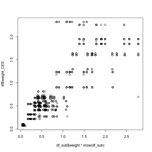
15 / 19
For more information on creating weights.
- Complex Surveys: a guide to analysis using R
- Applied Survey Data Analysis
- https://medium.com/pew-research-center-decoded/weighting-survey-data-with-the-pewmethods-r-package-d040afb0d2c2
16 / 19
When to use weights ?
- As a heuristic, it's ok to use them all the time.
- Always use them for description (for inferring a proportion from the sample to a population).
- Unclear when running regressions. See :https://www.jstor.org/stable/24735988#metadata_info_tab_contents
- If you run a regression where you control weighting variables, it's ok not to use weights.
17 / 19
Let's look at code Weights Example.R
18 / 19
- https://www.worldvaluessurvey.org/WVSDocumentationWV7.jsp
- https://electionstudies.org/data-center/2020-time-series-study/ (need to register)
- https://mccourt.georgetown.edu/master-of-science-in-data-science-for-public-policy/data-science-community/public-policy-data-sets-and-resources/
- https://medium.com/metapolicy/how-do-you-practice-data-science-b4c9df59bc9c
19 / 19