Introduction to R, the tidyverse way
SSMW 2022 University of Toronto
Justin Savoie
Acknowledgments
Thanks to Thomas Mock, Customer Enablement Lead at RStudio.
https://www.youtube.com/watch?v=MKwyauo8nSI&ab_channel=ThomasMock
Some parts of my presentation are inspired from his.
This presentation is available at https://www.justinsavoie.com/ssmw2022
Today's agenda
R and RStudio
- Writing code
- File manipulation
- Package control
R coding basics
- Math
- Assignment
- Functions
- Load and install packages
The tidyverse
- Read data in with readr
- Tidy data with tidyr
- Transform data with dplyr
Putting it together: two examples
- cleaning data; linear model with predicted values and marginal effects
- working with text from SCC cases
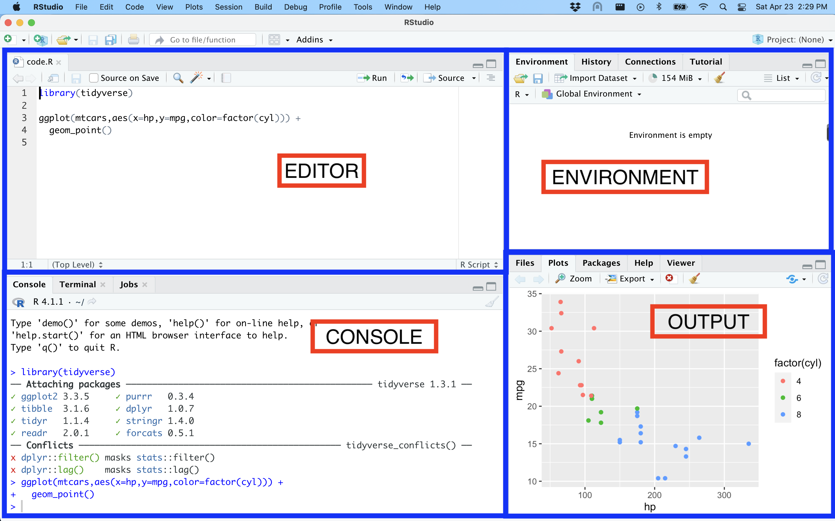
R and RStudio
- R is a programming language for statistical computing and graphics
- RStudio is an IDE (integrated development environment)
- A place to write:
- Console
- R scripts
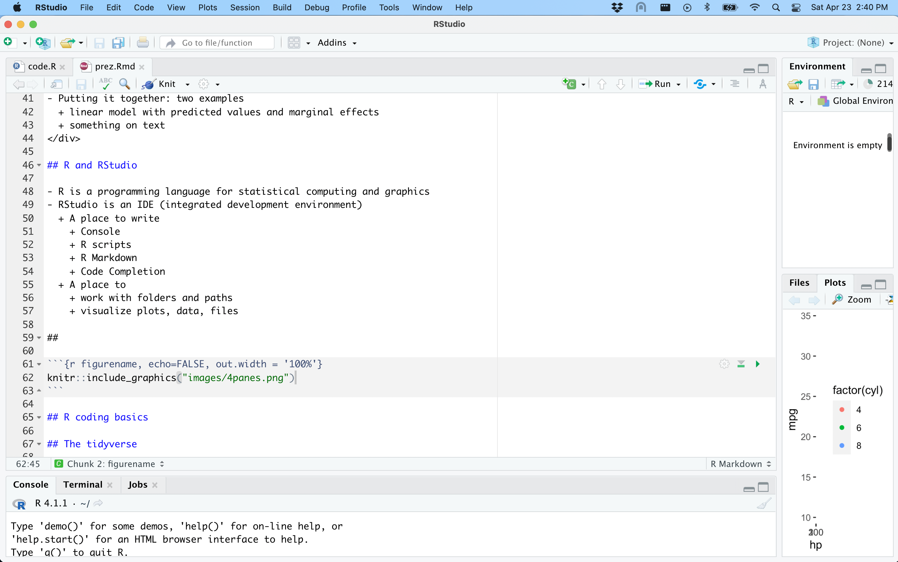
- R Markdown
- Code completion
- A place to:
- work with folders and paths
- visualize plots, data, files
Common mistakes


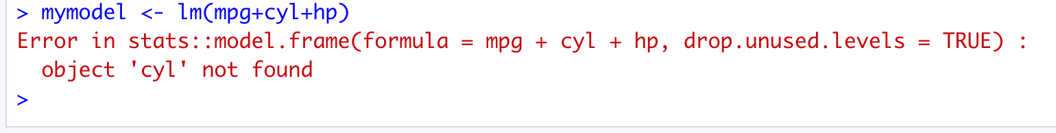
Error messages are usually informative.
You can also google the error message.
R coding basics (before tidyverse)
R coding basics
Assignment
x <- 2.5y <- 10z <- x*yz## [1] 25zz <- z + 2 *xzz## [1] 30x1 <- c(2,3,4,10,12,46)x2 <- c(-1,3,4,10,5,3)x1+x2## [1] 1 6 8 20 17 49x1 <- c(2,3,4,10,12,46)x2 <- c(-1,3,4,10,5,3,1,1,1.5)x1+x2## Warning in x1 + x2: longer object length is not a multiple of shorter object## length## [1] 1.0 6.0 8.0 20.0 17.0 49.0 3.0 4.0 5.5Dataframes
my_dataframe <- data.frame(x=c(1,2,3),y=c(3.5,4.5,5.5))my_dataframe## x y## 1 1 3.5## 2 2 4.5## 3 3 5.5head(mtcars)## mpg cyl disp hp drat wt qsec vs am gear carb## Mazda RX4 21.0 6 160 110 3.90 2.620 16.46 0 1 4 4## Mazda RX4 Wag 21.0 6 160 110 3.90 2.875 17.02 0 1 4 4## Datsun 710 22.8 4 108 93 3.85 2.320 18.61 1 1 4 1## Hornet 4 Drive 21.4 6 258 110 3.08 3.215 19.44 1 0 3 1## Hornet Sportabout 18.7 8 360 175 3.15 3.440 17.02 0 0 3 2## Valiant 18.1 6 225 105 2.76 3.460 20.22 1 0 3 1Functions
mean(c(2,3,4))## [1] 3random_vector<- rnorm(n=100,mean=0,sd=1)mean(random_vector)## [1] 0.1090938sd(random_vector)## [1] 0.9015466IQR(random_vector)## [1] 1.265599summary(random_vector)## Min. 1st Qu. Median Mean 3rd Qu. Max. ## -2.8532 -0.5379 0.1892 0.1091 0.7277 2.3159set.seed(232)random_vector <- rnorm(n=5,mean=0,sd=1)set.seed(232)random_vector <- rnorm(5,0,1)mean(x=random_vector)## [1] 0.233712mean(random_vector)## [1] 0.233712mtcars$cyl[1:5]## [1] 6 6 4 6 8my_quadratic_function <- function(x){ return(x^2+6*x+14.5)}my_quadratic_function(mtcars$cyl[1:5])## [1] 86.5 86.5 54.5 86.5 126.5mtcars$cylQUADRATIC <- my_quadratic_function(mtcars$cyl)head(mtcars,3)## mpg cyl disp hp drat wt qsec vs am gear carb cylQUADRATIC## Mazda RX4 21.0 6 160 110 3.90 2.620 16.46 0 1 4 4 86.5## Mazda RX4 Wag 21.0 6 160 110 3.90 2.875 17.02 0 1 4 4 86.5## Datsun 710 22.8 4 108 93 3.85 2.320 18.61 1 1 4 1 54.5Other useful functions
seq(from=1,to=3.5,by=0.5)## [1] 1.0 1.5 2.0 2.5 3.0 3.5seq(from=1,to=3.5,by=0.51)## [1] 1.00 1.51 2.02 2.53 3.04seq(from=-2,to=2,length.out=7)## [1] -2.0000000 -1.3333333 -0.6666667 0.0000000 0.6666667 1.3333333 2.0000000Other useful functions
table(mtcars$cyl)## ## 4 6 8 ## 11 7 14ifelse(c(3,3,6,8)>5,1,0)## [1] 0 0 1 1Other useful functions
plot(mtcars$mpg,mtcars$hp)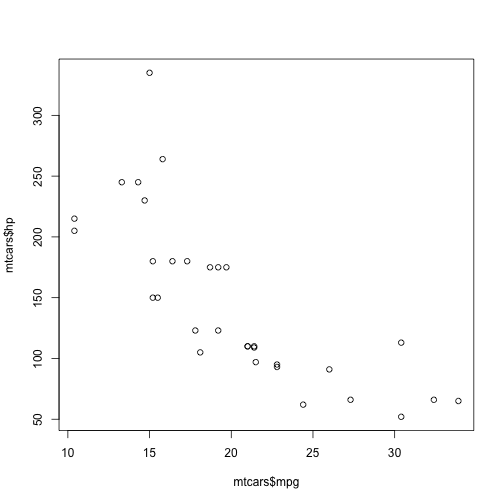
indexing
x <- c(1,2,3)x[2]## [1] 2x[2:3]## [1] 2 3mtcars$mpg[c(1,3)]## [1] 21.0 22.8indexing
mtcars[1:3,4:5]## hp drat## Mazda RX4 110 3.90## Mazda RX4 Wag 110 3.90## Datsun 710 93 3.85indexing
x[3] <- NAx## [1] 1 2 NAmtcars$mpg[mtcars$mpg>20]## [1] 21.0 21.0 22.8 21.4 24.4 22.8 32.4 30.4 33.9 21.5 27.3 26.0 30.4 21.4indexing
x <- mtcars$mpgx## [1] 21.0 21.0 22.8 21.4 18.7 18.1 14.3 24.4 22.8 19.2 17.8 16.4 17.3 15.2 10.4## [16] 10.4 14.7 32.4 30.4 33.9 21.5 15.5 15.2 13.3 19.2 27.3 26.0 30.4 15.8 19.7## [31] 15.0 21.4x[x>20] <- 1000x## [1] 1000.0 1000.0 1000.0 1000.0 18.7 18.1 14.3 1000.0 1000.0 19.2## [11] 17.8 16.4 17.3 15.2 10.4 10.4 14.7 1000.0 1000.0 1000.0## [21] 1000.0 15.5 15.2 13.3 19.2 1000.0 1000.0 1000.0 15.8 19.7## [31] 15.0 1000.0logical operators
2>3 # 2 is bigger than 3## [1] FALSE3>2 # 3 is bigger than 2## [1] TRUE2==2 # 2 is equal to 2## [1] TRUE2.00000001==2## [1] FALSE3!=2 # 3 is not equal to 2## [1] TRUElogical operators
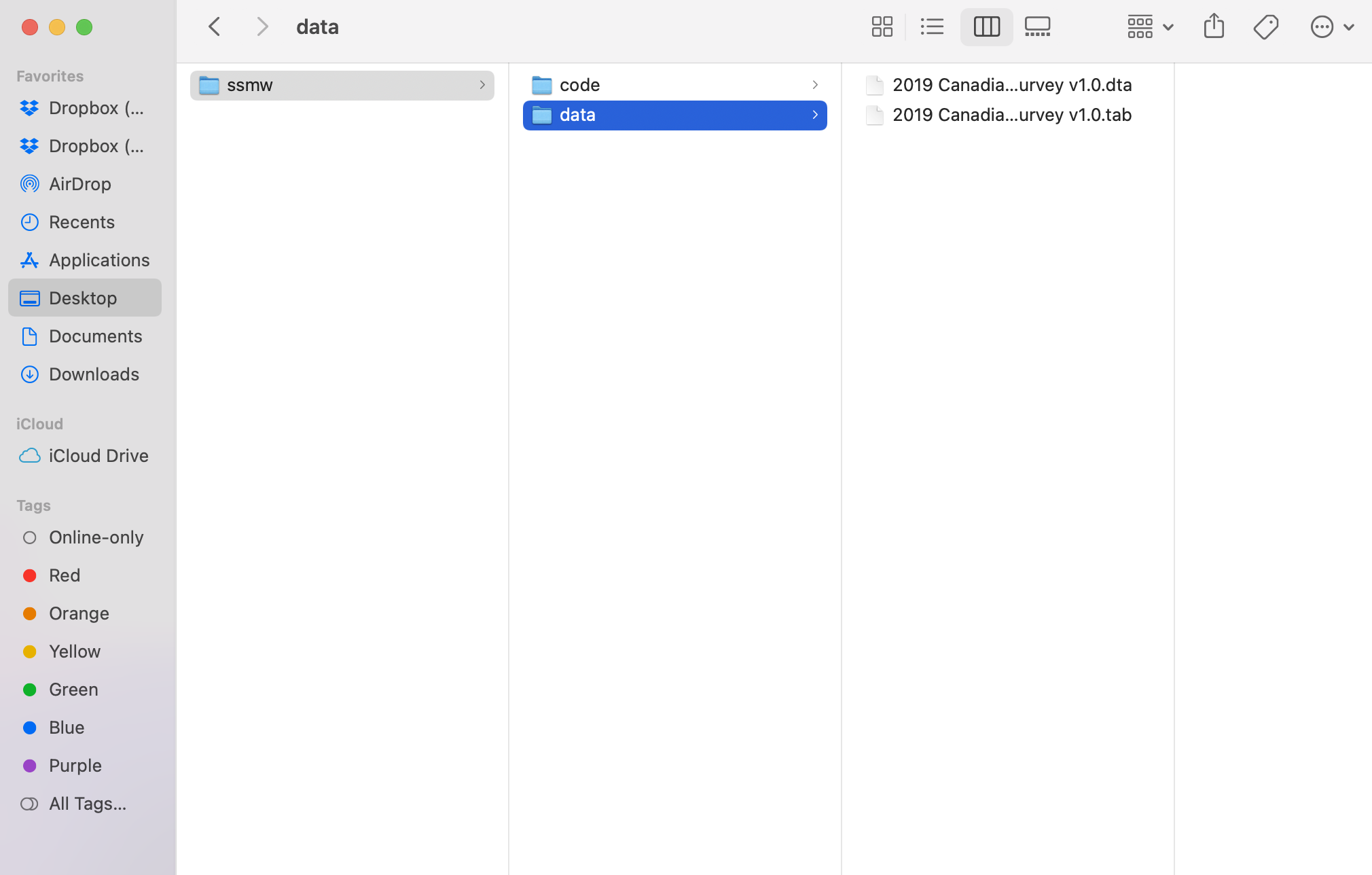
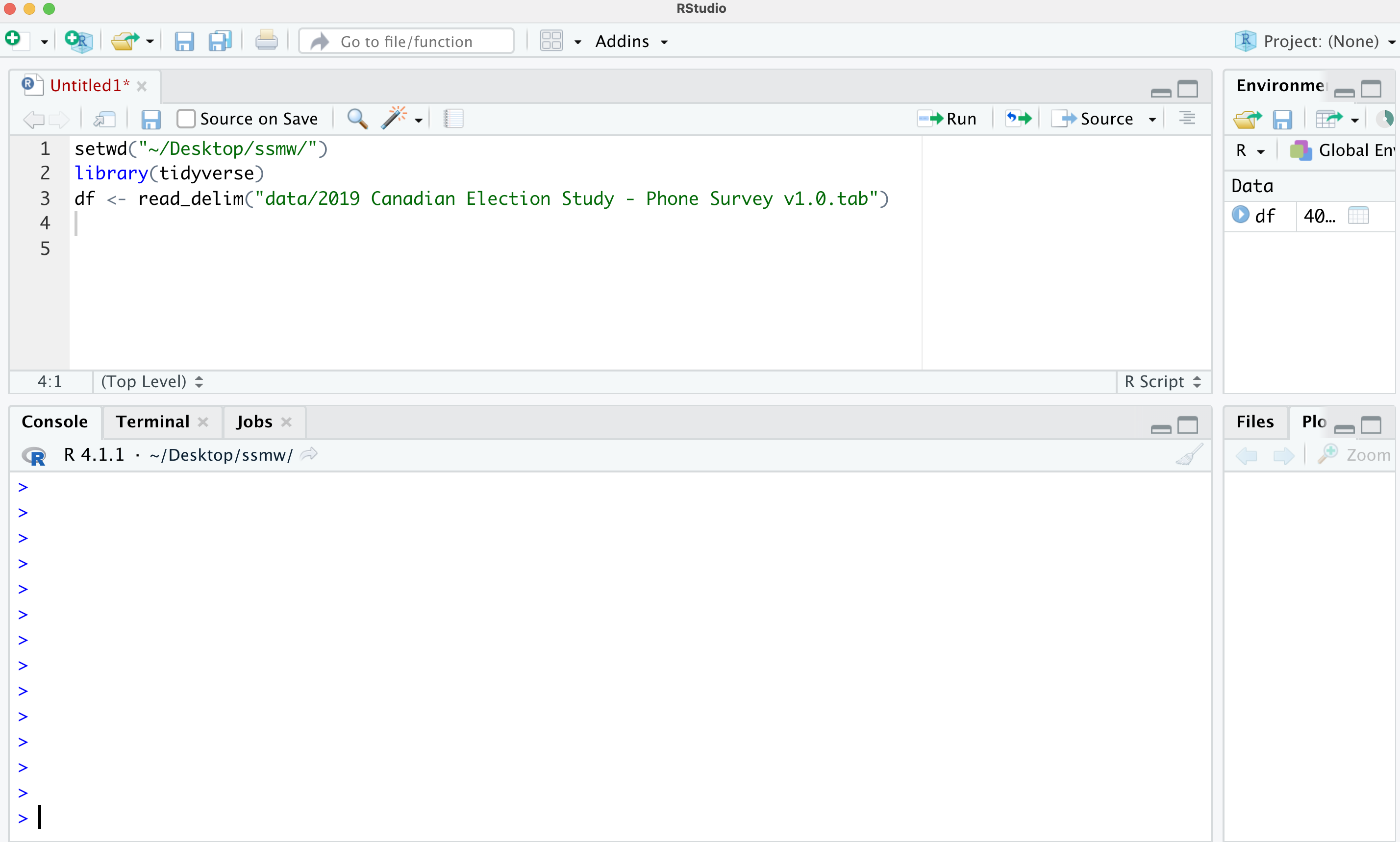
4 %in% c(2,4,5) # 4 is in the vector## [1] TRUE!(4 %in% c(2,4,5)) # 4 is not in the vector## [1] FALSE(5==6|6==6) # 5 or 6 is equal to 6## [1] TRUE(5==5&6==7) ### [1] FALSEis.na(c(2,3,NA)) # value is NA## [1] FALSE FALSE TRUEworking directory
my_data <- read_delim("/Users/justinsavoie/Downloads/ 2019 Canadian Election Study - Phone Survey v1.0.tab")setwd("~/Dropbox (Personal)/UofT/thisprojectimworkingon/")my_data <- read_delim("/data/ 2019 Canadian Election Study - Phone Survey v1.0.tab")To know a file's location:
on mac: cmd-i on file and copy 'where'
on pc: right click file and copy 'property'
working directory
working directory
The %>% (the 'pipe') and intro to tidyverse
did_something <- do_something(data)did_another_thing <- do_another_thing(did_something)do_last_thing <- do_last_thing(did_another_thing)final_thing <- do_last_thing( do_another_thing( do_something(data) ))final_thing <- data %>% do_something() %>% do_another_thing() %>% do_last_thing()The %>%
mean(c(1,2,3));## [1] 2c(1,2,3) %>% mean()## [1] 2The %>%
xplus6 <- function(x) x+6xminus2 <- function(x) x+2xtotwothird <- function(x) x^(2/3)my_vector <- c(3,4,2)my_vector %>% xplus6() %>% xminus2() %>% xtotwothird() %>% mean()## [1] 4.943053mean(xtotwothird(xminus2(xplus6(my_vector))))## [1] 4.943053The %>%
do_something(data) is equivalent to:
- data %>% do_something(data=.)
- data %>% do_something(.)
- data %>% do_something()
The %>%

ces <- read_csv("https://www.justinsavoie.com/data/dataces1.txt")head(ces)## # A tibble: 6 × 9## q2_birthyear q3_gender q4_province q6_satisfied_democracy q9_interest_elect…## <dbl> <chr> <chr> <chr> <chr> ## 1 1963 (1) Male (5) Quebec (3) Not very satisfied (8) ## 2 1973 (1) Male (5) Quebec (2) Fairly satisfied (10) Great deal o…## 3 1994 (1) Male (5) Quebec (1) Very satisfied (10) Great deal o…## 4 2000 (1) Male (5) Quebec (2) Fairly satisfied (6) ## 5 1984 (1) Male (5) Quebec (4) Not satisfied at all (10) Great deal o…## 6 1939 (1) Male (5) Quebec (3) Not very satisfied (10) Great deal o…## # … with 4 more variables: q10_certain_vote <chr>, q11_vote_intention <chr>,## # q14_feeling_liberal_party <dbl>, q15_feeling_cons_party <dbl>The %>%
ces %>% filter(q4_province=="(5) Quebec") %>% group_by(q3_gender) %>% summarise(mean_birthyear=mean(q2_birthyear), sd=sd(q2_birthyear))## # A tibble: 2 × 3## q3_gender mean_birthyear sd## <chr> <dbl> <dbl>## 1 (1) Male 1972. 15.9## 2 (2) Female 1970. 16.4The %>%
ces %>% group_by(q4_province,q3_gender) %>% summarise(mean_birthyear=mean(q2_birthyear), sd=sd(q2_birthyear)) %>% head(5)## `summarise()` has grouped output by 'q4_province'. You can override using the## `.groups` argument.## # A tibble: 5 × 4## # Groups: q4_province [2]## q4_province q3_gender mean_birthyear sd## <chr> <chr> <dbl> <dbl>## 1 (1) Newfoundland and Labrador (1) Male 1967. 15.7## 2 (1) Newfoundland and Labrador (2) Female 1965. 16.9## 3 (10) British Columbia (1) Male 1967. 17.3## 4 (10) British Columbia (2) Female 1966. 16.6## 5 (10) British Columbia (3) Other 1992 NAThe tidyverse
The tidyverse
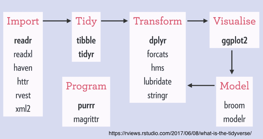
The tidyverse is an opinionated collection of R packages designed for data science.
All packages share an underlying design philosophy, grammar, and data structures.
tidyverse is a R package. But it's also a package of packages.
Core packages:
readr, tidyr, dplyr, ggplot2
tidyverse

tidyverse

Statistical inference using the tidyverse

tidyverse
Install and load packages
- Install package once on your computer.
install.packages('tidyverse')- Each time you run R, load the package.
library(tidyverse)tidyverse vs Base R
- People often contrast tidyverse and "base R"
- Many things can be done either in base R and with tidyverse
- Of course in practice, people use both. In particular: you need base R when you use the tidyverse for all the basic stuff.
read.csv("...")read_csv("...")plot(data$x,data$y)ggplot(data,aes(x=x,y=y)) + geom_point()tidyverse vs Base R
tapply(mtcars$mpg,mtcars$cyl,mean)## 4 6 8 ## 26.66364 19.74286 15.10000mtcars %>% group_by(cyl) %>% summarise(mean(mpg))## # A tibble: 3 × 2## cyl `mean(mpg)`## <dbl> <dbl>## 1 4 26.7## 2 6 19.7## 3 8 15.1tidyverse vs Base R
mtcars$new_var <- rnorm(nrow(mtcars),0,1)mtcars <- mtcars %>% mutate(new_var=rnorm(nrow(.),0,1))tidyverse core principles
- Built about two-dimensional data (data.frame or tibble)
- Built around tidy data
- Each variable in it's own column
- Each observation in its own row
- Each type of observational units forms a table
Tidy data
head(ces)## # A tibble: 6 × 9## q2_birthyear q3_gender q4_province q6_satisfied_democracy q9_interest_elect…## <dbl> <chr> <chr> <chr> <chr> ## 1 1963 (1) Male (5) Quebec (3) Not very satisfied (8) ## 2 1973 (1) Male (5) Quebec (2) Fairly satisfied (10) Great deal o…## 3 1994 (1) Male (5) Quebec (1) Very satisfied (10) Great deal o…## 4 2000 (1) Male (5) Quebec (2) Fairly satisfied (6) ## 5 1984 (1) Male (5) Quebec (4) Not satisfied at all (10) Great deal o…## 6 1939 (1) Male (5) Quebec (3) Not very satisfied (10) Great deal o…## # … with 4 more variables: q10_certain_vote <chr>, q11_vote_intention <chr>,## # q14_feeling_liberal_party <dbl>, q15_feeling_cons_party <dbl>Untidy data
(untidy_df <- tibble(age=18:30, male_2016=round(rnorm(13,50000,5000)), female_2016=round(rnorm(13,50000,5000)), male_2017=round(rnorm(13,50000,5000)), female_2017=round(rnorm(13,50000,5000)), male_2018=round(rnorm(13,50000,5000)), female_2018=round(rnorm(13,50000,5000)))) %>% head(10)## # A tibble: 10 × 7## age male_2016 female_2016 male_2017 female_2017 male_2018 female_2018## <int> <dbl> <dbl> <dbl> <dbl> <dbl> <dbl>## 1 18 52579 52796 55592 50408 50659 49530## 2 19 52374 53110 56601 53242 45912 52298## 3 20 44102 48351 53827 55603 46277 54563## 4 21 50885 38245 38620 45510 54871 58411## 5 22 44634 45495 51560 45302 53563 52324## 6 23 50467 46760 51060 48077 39407 56501## 7 24 51462 47773 50152 44989 53284 54753## 8 25 54106 46685 47309 50160 57431 59393## 9 26 57848 46243 44781 47118 48008 52496## 10 27 56968 45185 59887 56179 48006 53883Tidy data
(tidy_df <- untidy_df %>% pivot_longer(-age,names_to = c("gender","year"), values_to = "value",names_sep = "_"))## # A tibble: 78 × 4## age gender year value## <int> <chr> <chr> <dbl>## 1 18 male 2016 52579## 2 18 female 2016 52796## 3 18 male 2017 55592## 4 18 female 2017 50408## 5 18 male 2018 50659## 6 18 female 2018 49530## 7 19 male 2016 52374## 8 19 female 2016 53110## 9 19 male 2017 56601## 10 19 female 2017 53242## # … with 68 more rowsRead data
Read in data with readr, haven, readxl.
I've also used readstata13 which is not in tidyverse.
readrread_csv(),read_tsv(),read_delim()
havenread_sas(),read_spss(),read_stata()
readxlread_xls(),read_xlsx(),read_excel()
For example:
df <- read_csv("~/Desktop/mydata.csv")dplyr package
6 main verbs
filter()keep only certain rowsarrange()order rows by order in a variableselect()keep only certain variablesmutate()create a variablegroup_by()group by values in a variablesummarise()summarise e.g. mean, sd etc.
simple functions
pull()extract one variable and make it vectorn()andcount()glimpse()give summary of data
dplyr package
advanced iterations
summarize_atsummarise on many variablesmutate_atcreate/modify many variablessummarize_allmutate_all
for more info
- dplyr.tidyverse.org
- R for Data Science
- Stack Overflow

mtcars dataset
class(mtcars)## [1] "data.frame"mtcars_tbl <- as_tibble(mtcars)class(mtcars_tbl)## [1] "tbl_df" "tbl" "data.frame"mtcars dataset
mtcars## mpg cyl disp hp drat wt qsec vs am gear carb## Mazda RX4 21.0 6 160.0 110 3.90 2.620 16.46 0 1 4 4## Mazda RX4 Wag 21.0 6 160.0 110 3.90 2.875 17.02 0 1 4 4## Datsun 710 22.8 4 108.0 93 3.85 2.320 18.61 1 1 4 1## Hornet 4 Drive 21.4 6 258.0 110 3.08 3.215 19.44 1 0 3 1## Hornet Sportabout 18.7 8 360.0 175 3.15 3.440 17.02 0 0 3 2## Valiant 18.1 6 225.0 105 2.76 3.460 20.22 1 0 3 1## Duster 360 14.3 8 360.0 245 3.21 3.570 15.84 0 0 3 4## Merc 240D 24.4 4 146.7 62 3.69 3.190 20.00 1 0 4 2## Merc 230 22.8 4 140.8 95 3.92 3.150 22.90 1 0 4 2## Merc 280 19.2 6 167.6 123 3.92 3.440 18.30 1 0 4 4## Merc 280C 17.8 6 167.6 123 3.92 3.440 18.90 1 0 4 4## Merc 450SE 16.4 8 275.8 180 3.07 4.070 17.40 0 0 3 3## Merc 450SL 17.3 8 275.8 180 3.07 3.730 17.60 0 0 3 3## Merc 450SLC 15.2 8 275.8 180 3.07 3.780 18.00 0 0 3 3## Cadillac Fleetwood 10.4 8 472.0 205 2.93 5.250 17.98 0 0 3 4## Lincoln Continental 10.4 8 460.0 215 3.00 5.424 17.82 0 0 3 4## Chrysler Imperial 14.7 8 440.0 230 3.23 5.345 17.42 0 0 3 4## Fiat 128 32.4 4 78.7 66 4.08 2.200 19.47 1 1 4 1## Honda Civic 30.4 4 75.7 52 4.93 1.615 18.52 1 1 4 2## Toyota Corolla 33.9 4 71.1 65 4.22 1.835 19.90 1 1 4 1## Toyota Corona 21.5 4 120.1 97 3.70 2.465 20.01 1 0 3 1## Dodge Challenger 15.5 8 318.0 150 2.76 3.520 16.87 0 0 3 2## AMC Javelin 15.2 8 304.0 150 3.15 3.435 17.30 0 0 3 2## Camaro Z28 13.3 8 350.0 245 3.73 3.840 15.41 0 0 3 4## Pontiac Firebird 19.2 8 400.0 175 3.08 3.845 17.05 0 0 3 2## Fiat X1-9 27.3 4 79.0 66 4.08 1.935 18.90 1 1 4 1## Porsche 914-2 26.0 4 120.3 91 4.43 2.140 16.70 0 1 5 2## Lotus Europa 30.4 4 95.1 113 3.77 1.513 16.90 1 1 5 2## Ford Pantera L 15.8 8 351.0 264 4.22 3.170 14.50 0 1 5 4## Ferrari Dino 19.7 6 145.0 175 3.62 2.770 15.50 0 1 5 6## Maserati Bora 15.0 8 301.0 335 3.54 3.570 14.60 0 1 5 8## Volvo 142E 21.4 4 121.0 109 4.11 2.780 18.60 1 1 4 2mtcars dataset
mtcars_tbl## # A tibble: 32 × 11## mpg cyl disp hp drat wt qsec vs am gear carb## <dbl> <dbl> <dbl> <dbl> <dbl> <dbl> <dbl> <dbl> <dbl> <dbl> <dbl>## 1 21 6 160 110 3.9 2.62 16.5 0 1 4 4## 2 21 6 160 110 3.9 2.88 17.0 0 1 4 4## 3 22.8 4 108 93 3.85 2.32 18.6 1 1 4 1## 4 21.4 6 258 110 3.08 3.22 19.4 1 0 3 1## 5 18.7 8 360 175 3.15 3.44 17.0 0 0 3 2## 6 18.1 6 225 105 2.76 3.46 20.2 1 0 3 1## 7 14.3 8 360 245 3.21 3.57 15.8 0 0 3 4## 8 24.4 4 147. 62 3.69 3.19 20 1 0 4 2## 9 22.8 4 141. 95 3.92 3.15 22.9 1 0 4 2## 10 19.2 6 168. 123 3.92 3.44 18.3 1 0 4 4## # … with 22 more rowsmtcars dataset
mtcars_tbl <- mtcars %>% mutate(name=row.names(.)) %>% as_tibble()head(mtcars_tbl,3)## # A tibble: 3 × 12## mpg cyl disp hp drat wt qsec vs am gear carb name ## <dbl> <dbl> <dbl> <dbl> <dbl> <dbl> <dbl> <dbl> <dbl> <dbl> <dbl> <chr> ## 1 21 6 160 110 3.9 2.62 16.5 0 1 4 4 Mazda RX4 ## 2 21 6 160 110 3.9 2.88 17.0 0 1 4 4 Mazda RX4 W…## 3 22.8 4 108 93 3.85 2.32 18.6 1 1 4 1 Datsun 710mtcars dataset
mtcars <- mtcars_tbldplyr::slice()
mtcars %>% slice(c(1,2,3))## # A tibble: 3 × 12## mpg cyl disp hp drat wt qsec vs am gear carb name ## <dbl> <dbl> <dbl> <dbl> <dbl> <dbl> <dbl> <dbl> <dbl> <dbl> <dbl> <chr> ## 1 21 6 160 110 3.9 2.62 16.5 0 1 4 4 Mazda RX4 ## 2 21 6 160 110 3.9 2.88 17.0 0 1 4 4 Mazda RX4 W…## 3 22.8 4 108 93 3.85 2.32 18.6 1 1 4 1 Datsun 710dplyr::slice()
mtcars %>% slice(c(1,4,5))## # A tibble: 3 × 12## mpg cyl disp hp drat wt qsec vs am gear carb name ## <dbl> <dbl> <dbl> <dbl> <dbl> <dbl> <dbl> <dbl> <dbl> <dbl> <dbl> <chr> ## 1 21 6 160 110 3.9 2.62 16.5 0 1 4 4 Mazda RX4 ## 2 21.4 6 258 110 3.08 3.22 19.4 1 0 3 1 Hornet 4 Dr…## 3 18.7 8 360 175 3.15 3.44 17.0 0 0 3 2 Hornet Spor…dplyr::glimpse()
mtcars %>% glimpse()## Rows: 32## Columns: 12## $ mpg <dbl> 21.0, 21.0, 22.8, 21.4, 18.7, 18.1, 14.3, 24.4, 22.8, 19.2, 17.8,…## $ cyl <dbl> 6, 6, 4, 6, 8, 6, 8, 4, 4, 6, 6, 8, 8, 8, 8, 8, 8, 4, 4, 4, 4, 8,…## $ disp <dbl> 160.0, 160.0, 108.0, 258.0, 360.0, 225.0, 360.0, 146.7, 140.8, 16…## $ hp <dbl> 110, 110, 93, 110, 175, 105, 245, 62, 95, 123, 123, 180, 180, 180…## $ drat <dbl> 3.90, 3.90, 3.85, 3.08, 3.15, 2.76, 3.21, 3.69, 3.92, 3.92, 3.92,…## $ wt <dbl> 2.620, 2.875, 2.320, 3.215, 3.440, 3.460, 3.570, 3.190, 3.150, 3.…## $ qsec <dbl> 16.46, 17.02, 18.61, 19.44, 17.02, 20.22, 15.84, 20.00, 22.90, 18…## $ vs <dbl> 0, 0, 1, 1, 0, 1, 0, 1, 1, 1, 1, 0, 0, 0, 0, 0, 0, 1, 1, 1, 1, 0,…## $ am <dbl> 1, 1, 1, 0, 0, 0, 0, 0, 0, 0, 0, 0, 0, 0, 0, 0, 0, 1, 1, 1, 0, 0,…## $ gear <dbl> 4, 4, 4, 3, 3, 3, 3, 4, 4, 4, 4, 3, 3, 3, 3, 3, 3, 4, 4, 4, 3, 3,…## $ carb <dbl> 4, 4, 1, 1, 2, 1, 4, 2, 2, 4, 4, 3, 3, 3, 4, 4, 4, 1, 2, 1, 1, 2,…## $ name <chr> "Mazda RX4", "Mazda RX4 Wag", "Datsun 710", "Hornet 4 Drive", "Ho…dplyr::filter()
mtcars %>% filter(cyl==4)## # A tibble: 11 × 12## mpg cyl disp hp drat wt qsec vs am gear carb name ## <dbl> <dbl> <dbl> <dbl> <dbl> <dbl> <dbl> <dbl> <dbl> <dbl> <dbl> <chr> ## 1 22.8 4 108 93 3.85 2.32 18.6 1 1 4 1 Datsun 710 ## 2 24.4 4 147. 62 3.69 3.19 20 1 0 4 2 Merc 240D ## 3 22.8 4 141. 95 3.92 3.15 22.9 1 0 4 2 Merc 230 ## 4 32.4 4 78.7 66 4.08 2.2 19.5 1 1 4 1 Fiat 128 ## 5 30.4 4 75.7 52 4.93 1.62 18.5 1 1 4 2 Honda Civic## 6 33.9 4 71.1 65 4.22 1.84 19.9 1 1 4 1 Toyota Cor…## 7 21.5 4 120. 97 3.7 2.46 20.0 1 0 3 1 Toyota Cor…## 8 27.3 4 79 66 4.08 1.94 18.9 1 1 4 1 Fiat X1-9 ## 9 26 4 120. 91 4.43 2.14 16.7 0 1 5 2 Porsche 91…## 10 30.4 4 95.1 113 3.77 1.51 16.9 1 1 5 2 Lotus Euro…## 11 21.4 4 121 109 4.11 2.78 18.6 1 1 4 2 Volvo 142Edplyr::filter()
mtcars %>% filter(cyl!=4)## # A tibble: 21 × 12## mpg cyl disp hp drat wt qsec vs am gear carb name ## <dbl> <dbl> <dbl> <dbl> <dbl> <dbl> <dbl> <dbl> <dbl> <dbl> <dbl> <chr> ## 1 21 6 160 110 3.9 2.62 16.5 0 1 4 4 Mazda RX4 ## 2 21 6 160 110 3.9 2.88 17.0 0 1 4 4 Mazda RX4 …## 3 21.4 6 258 110 3.08 3.22 19.4 1 0 3 1 Hornet 4 D…## 4 18.7 8 360 175 3.15 3.44 17.0 0 0 3 2 Hornet Spo…## 5 18.1 6 225 105 2.76 3.46 20.2 1 0 3 1 Valiant ## 6 14.3 8 360 245 3.21 3.57 15.8 0 0 3 4 Duster 360 ## 7 19.2 6 168. 123 3.92 3.44 18.3 1 0 4 4 Merc 280 ## 8 17.8 6 168. 123 3.92 3.44 18.9 1 0 4 4 Merc 280C ## 9 16.4 8 276. 180 3.07 4.07 17.4 0 0 3 3 Merc 450SE ## 10 17.3 8 276. 180 3.07 3.73 17.6 0 0 3 3 Merc 450SL ## # … with 11 more rowsdplyr::filter()
mtcars %>% filter(cyl %in% c(4,6))## # A tibble: 18 × 12## mpg cyl disp hp drat wt qsec vs am gear carb name ## <dbl> <dbl> <dbl> <dbl> <dbl> <dbl> <dbl> <dbl> <dbl> <dbl> <dbl> <chr> ## 1 21 6 160 110 3.9 2.62 16.5 0 1 4 4 Mazda RX4 ## 2 21 6 160 110 3.9 2.88 17.0 0 1 4 4 Mazda RX4 …## 3 22.8 4 108 93 3.85 2.32 18.6 1 1 4 1 Datsun 710 ## 4 21.4 6 258 110 3.08 3.22 19.4 1 0 3 1 Hornet 4 D…## 5 18.1 6 225 105 2.76 3.46 20.2 1 0 3 1 Valiant ## 6 24.4 4 147. 62 3.69 3.19 20 1 0 4 2 Merc 240D ## 7 22.8 4 141. 95 3.92 3.15 22.9 1 0 4 2 Merc 230 ## 8 19.2 6 168. 123 3.92 3.44 18.3 1 0 4 4 Merc 280 ## 9 17.8 6 168. 123 3.92 3.44 18.9 1 0 4 4 Merc 280C ## 10 32.4 4 78.7 66 4.08 2.2 19.5 1 1 4 1 Fiat 128 ## 11 30.4 4 75.7 52 4.93 1.62 18.5 1 1 4 2 Honda Civic## 12 33.9 4 71.1 65 4.22 1.84 19.9 1 1 4 1 Toyota Cor…## 13 21.5 4 120. 97 3.7 2.46 20.0 1 0 3 1 Toyota Cor…## 14 27.3 4 79 66 4.08 1.94 18.9 1 1 4 1 Fiat X1-9 ## 15 26 4 120. 91 4.43 2.14 16.7 0 1 5 2 Porsche 91…## 16 30.4 4 95.1 113 3.77 1.51 16.9 1 1 5 2 Lotus Euro…## 17 19.7 6 145 175 3.62 2.77 15.5 0 1 5 6 Ferrari Di…## 18 21.4 4 121 109 4.11 2.78 18.6 1 1 4 2 Volvo 142Edplyr::select()
select(mtcars,hp,mpg,cyl)## # A tibble: 32 × 3## hp mpg cyl## <dbl> <dbl> <dbl>## 1 110 21 6## 2 110 21 6## 3 93 22.8 4## 4 110 21.4 6## 5 175 18.7 8## 6 105 18.1 6## 7 245 14.3 8## 8 62 24.4 4## 9 95 22.8 4## 10 123 19.2 6## # … with 22 more rowsdplyr::select()
mtcars %>% select(-mpg)## # A tibble: 32 × 11## cyl disp hp drat wt qsec vs am gear carb name ## <dbl> <dbl> <dbl> <dbl> <dbl> <dbl> <dbl> <dbl> <dbl> <dbl> <chr> ## 1 6 160 110 3.9 2.62 16.5 0 1 4 4 Mazda RX4 ## 2 6 160 110 3.9 2.88 17.0 0 1 4 4 Mazda RX4 Wag ## 3 4 108 93 3.85 2.32 18.6 1 1 4 1 Datsun 710 ## 4 6 258 110 3.08 3.22 19.4 1 0 3 1 Hornet 4 Drive ## 5 8 360 175 3.15 3.44 17.0 0 0 3 2 Hornet Sportabout## 6 6 225 105 2.76 3.46 20.2 1 0 3 1 Valiant ## 7 8 360 245 3.21 3.57 15.8 0 0 3 4 Duster 360 ## 8 4 147. 62 3.69 3.19 20 1 0 4 2 Merc 240D ## 9 4 141. 95 3.92 3.15 22.9 1 0 4 2 Merc 230 ## 10 6 168. 123 3.92 3.44 18.3 1 0 4 4 Merc 280 ## # … with 22 more rowsdplyr::select()
mtcars %>% select(starts_with("c"),starts_with("h"))## # A tibble: 32 × 3## cyl carb hp## <dbl> <dbl> <dbl>## 1 6 4 110## 2 6 4 110## 3 4 1 93## 4 6 1 110## 5 8 2 175## 6 6 1 105## 7 8 4 245## 8 4 2 62## 9 4 2 95## 10 6 4 123## # … with 22 more rowsdplyr::arrange()
mtcars %>% arrange(mpg)## # A tibble: 32 × 12## mpg cyl disp hp drat wt qsec vs am gear carb name ## <dbl> <dbl> <dbl> <dbl> <dbl> <dbl> <dbl> <dbl> <dbl> <dbl> <dbl> <chr> ## 1 10.4 8 472 205 2.93 5.25 18.0 0 0 3 4 Cadillac F…## 2 10.4 8 460 215 3 5.42 17.8 0 0 3 4 Lincoln Co…## 3 13.3 8 350 245 3.73 3.84 15.4 0 0 3 4 Camaro Z28 ## 4 14.3 8 360 245 3.21 3.57 15.8 0 0 3 4 Duster 360 ## 5 14.7 8 440 230 3.23 5.34 17.4 0 0 3 4 Chrysler I…## 6 15 8 301 335 3.54 3.57 14.6 0 1 5 8 Maserati B…## 7 15.2 8 276. 180 3.07 3.78 18 0 0 3 3 Merc 450SLC## 8 15.2 8 304 150 3.15 3.44 17.3 0 0 3 2 AMC Javelin## 9 15.5 8 318 150 2.76 3.52 16.9 0 0 3 2 Dodge Chal…## 10 15.8 8 351 264 4.22 3.17 14.5 0 1 5 4 Ford Pante…## # … with 22 more rowsdplyr::arrange()
mtcars %>% arrange(desc(mpg))## # A tibble: 32 × 12## mpg cyl disp hp drat wt qsec vs am gear carb name ## <dbl> <dbl> <dbl> <dbl> <dbl> <dbl> <dbl> <dbl> <dbl> <dbl> <dbl> <chr> ## 1 33.9 4 71.1 65 4.22 1.84 19.9 1 1 4 1 Toyota Cor…## 2 32.4 4 78.7 66 4.08 2.2 19.5 1 1 4 1 Fiat 128 ## 3 30.4 4 75.7 52 4.93 1.62 18.5 1 1 4 2 Honda Civic## 4 30.4 4 95.1 113 3.77 1.51 16.9 1 1 5 2 Lotus Euro…## 5 27.3 4 79 66 4.08 1.94 18.9 1 1 4 1 Fiat X1-9 ## 6 26 4 120. 91 4.43 2.14 16.7 0 1 5 2 Porsche 91…## 7 24.4 4 147. 62 3.69 3.19 20 1 0 4 2 Merc 240D ## 8 22.8 4 108 93 3.85 2.32 18.6 1 1 4 1 Datsun 710 ## 9 22.8 4 141. 95 3.92 3.15 22.9 1 0 4 2 Merc 230 ## 10 21.5 4 120. 97 3.7 2.46 20.0 1 0 3 1 Toyota Cor…## # … with 22 more rowsdplyr::arrange()
mtcars %>% arrange(desc(cyl),disp)## # A tibble: 32 × 12## mpg cyl disp hp drat wt qsec vs am gear carb name ## <dbl> <dbl> <dbl> <dbl> <dbl> <dbl> <dbl> <dbl> <dbl> <dbl> <dbl> <chr> ## 1 16.4 8 276. 180 3.07 4.07 17.4 0 0 3 3 Merc 450SE ## 2 17.3 8 276. 180 3.07 3.73 17.6 0 0 3 3 Merc 450SL ## 3 15.2 8 276. 180 3.07 3.78 18 0 0 3 3 Merc 450SLC## 4 15 8 301 335 3.54 3.57 14.6 0 1 5 8 Maserati B…## 5 15.2 8 304 150 3.15 3.44 17.3 0 0 3 2 AMC Javelin## 6 15.5 8 318 150 2.76 3.52 16.9 0 0 3 2 Dodge Chal…## 7 13.3 8 350 245 3.73 3.84 15.4 0 0 3 4 Camaro Z28 ## 8 15.8 8 351 264 4.22 3.17 14.5 0 1 5 4 Ford Pante…## 9 18.7 8 360 175 3.15 3.44 17.0 0 0 3 2 Hornet Spo…## 10 14.3 8 360 245 3.21 3.57 15.8 0 0 3 4 Duster 360 ## # … with 22 more rowsdplyr::mutate()
mtcars %>% mutate(hpsquare=hp^2) %>% select(mpg,cyl,disp,hp,hpsquare)## # A tibble: 32 × 5## mpg cyl disp hp hpsquare## <dbl> <dbl> <dbl> <dbl> <dbl>## 1 21 6 160 110 12100## 2 21 6 160 110 12100## 3 22.8 4 108 93 8649## 4 21.4 6 258 110 12100## 5 18.7 8 360 175 30625## 6 18.1 6 225 105 11025## 7 14.3 8 360 245 60025## 8 24.4 4 147. 62 3844## 9 22.8 4 141. 95 9025## 10 19.2 6 168. 123 15129## # … with 22 more rowsdplyr::mutate()
mtcars %>% mutate(randomnoise=rnorm(nrow(.),mean=0,sd=1), mpg_with_random_noise = mpg+randomnoise) %>% select(mpg,cyl,disp,randomnoise,mpg_with_random_noise)## # A tibble: 32 × 5## mpg cyl disp randomnoise mpg_with_random_noise## <dbl> <dbl> <dbl> <dbl> <dbl>## 1 21 6 160 -0.391 20.6## 2 21 6 160 3.10 24.1## 3 22.8 4 108 -1.88 20.9## 4 21.4 6 258 0.565 22.0## 5 18.7 8 360 1.31 20.0## 6 18.1 6 225 0.734 18.8## 7 14.3 8 360 -0.848 13.5## 8 24.4 4 147. 1.32 25.7## 9 22.8 4 141. -0.505 22.3## 10 19.2 6 168. -0.652 18.5## # … with 22 more rowsdplyr::mutate()
mtcars %>% mutate(cyl=factor(cyl,levels=c(4,6,8), labels=c("4 Cyl","6 Cyl","8 Cyl")))## # A tibble: 32 × 12## mpg cyl disp hp drat wt qsec vs am gear carb name ## <dbl> <fct> <dbl> <dbl> <dbl> <dbl> <dbl> <dbl> <dbl> <dbl> <dbl> <chr> ## 1 21 6 Cyl 160 110 3.9 2.62 16.5 0 1 4 4 Mazda RX4 ## 2 21 6 Cyl 160 110 3.9 2.88 17.0 0 1 4 4 Mazda RX4 …## 3 22.8 4 Cyl 108 93 3.85 2.32 18.6 1 1 4 1 Datsun 710 ## 4 21.4 6 Cyl 258 110 3.08 3.22 19.4 1 0 3 1 Hornet 4 D…## 5 18.7 8 Cyl 360 175 3.15 3.44 17.0 0 0 3 2 Hornet Spo…## 6 18.1 6 Cyl 225 105 2.76 3.46 20.2 1 0 3 1 Valiant ## 7 14.3 8 Cyl 360 245 3.21 3.57 15.8 0 0 3 4 Duster 360 ## 8 24.4 4 Cyl 147. 62 3.69 3.19 20 1 0 4 2 Merc 240D ## 9 22.8 4 Cyl 141. 95 3.92 3.15 22.9 1 0 4 2 Merc 230 ## 10 19.2 6 Cyl 168. 123 3.92 3.44 18.3 1 0 4 4 Merc 280 ## # … with 22 more rowsmore on factors
vect <- c("Much less","About the same","Much more")class(vect)## [1] "character"table(vect)## vect## About the same Much less Much more ## 1 1 1vect <- factor(vect,levels=c("Much less","About the same","Much more"))class(vect)## [1] "factor"table(vect)## vect## Much less About the same Much more ## 1 1 1more on factors
vect <- factor(vect,levels=c("Much less","About the same","Much more"), labels=c("ml","abs","mm"))vect## [1] ml abs mm ## Levels: ml abs mmas.numeric(vect)## [1] 1 2 3more on factors
vect <- 1:22factor(vect)## [1] 1 2 3 4 5 6 7 8 9 10 11 12 13 14 15 16 17 18 19 20 21 22## Levels: 1 2 3 4 5 6 7 8 9 10 11 12 13 14 15 16 17 18 19 20 21 22vect <- as.character(1:22)(fct_vect <- factor(vect))## [1] 1 2 3 4 5 6 7 8 9 10 11 12 13 14 15 16 17 18 19 20 21 22## Levels: 1 10 11 12 13 14 15 16 17 18 19 2 20 21 22 3 4 5 6 7 8 9as.numeric(fct_vect)## [1] 1 12 16 17 18 19 20 21 22 2 3 4 5 6 7 8 9 10 11 13 14 15more on factors
mtcars %>% mutate(cyl=factor(cyl,levels=c(4,6,8), labels=c("4 Cyl","6 Cyl","8 Cyl")), cyl2 = fct_recode(cyl,"Small"="4 Cyl", "Big"="6 Cyl", "Big"="8 Cyl")) %>% select(cyl,cyl2)## # A tibble: 32 × 2## cyl cyl2 ## <fct> <fct>## 1 6 Cyl Big ## 2 6 Cyl Big ## 3 4 Cyl Small## 4 6 Cyl Big ## 5 8 Cyl Big ## 6 6 Cyl Big ## 7 8 Cyl Big ## 8 4 Cyl Small## 9 4 Cyl Small## 10 6 Cyl Big ## # … with 22 more rowsmore on factors
temp <- mtcars %>% mutate(cyl_f=factor(cyl,levels=c(4,6,8), labels=c("4 Cyl","6 Cyl","8 Cyl")), cyl2 = fct_recode(cyl_f,"Small"="4 Cyl","Big"="6 Cyl","Big"="8 Cyl"), cyl2REV=fct_relevel(cyl2,"Big","Small"))table(temp$cyl2)## ## Small Big ## 11 21table(temp$cyl2REV)## ## Big Small ## 21 11dplyr::mutate()
mtcars %>% mutate(miles_per_liter = mpg*3.78, miles_per_gallon=miles_per_liter/3.78) %>% select(miles_per_liter,mpg,miles_per_gallon)## # A tibble: 32 × 3## miles_per_liter mpg miles_per_gallon## <dbl> <dbl> <dbl>## 1 79.4 21 21 ## 2 79.4 21 21 ## 3 86.2 22.8 22.8## 4 80.9 21.4 21.4## 5 70.7 18.7 18.7## 6 68.4 18.1 18.1## 7 54.1 14.3 14.3## 8 92.2 24.4 24.4## 9 86.2 22.8 22.8## 10 72.6 19.2 19.2## # … with 22 more rowsdplyr::group_by()
mtcars %>% group_by(cyl)## # A tibble: 32 × 12## # Groups: cyl [3]## mpg cyl disp hp drat wt qsec vs am gear carb name ## <dbl> <dbl> <dbl> <dbl> <dbl> <dbl> <dbl> <dbl> <dbl> <dbl> <dbl> <chr> ## 1 21 6 160 110 3.9 2.62 16.5 0 1 4 4 Mazda RX4 ## 2 21 6 160 110 3.9 2.88 17.0 0 1 4 4 Mazda RX4 …## 3 22.8 4 108 93 3.85 2.32 18.6 1 1 4 1 Datsun 710 ## 4 21.4 6 258 110 3.08 3.22 19.4 1 0 3 1 Hornet 4 D…## 5 18.7 8 360 175 3.15 3.44 17.0 0 0 3 2 Hornet Spo…## 6 18.1 6 225 105 2.76 3.46 20.2 1 0 3 1 Valiant ## 7 14.3 8 360 245 3.21 3.57 15.8 0 0 3 4 Duster 360 ## 8 24.4 4 147. 62 3.69 3.19 20 1 0 4 2 Merc 240D ## 9 22.8 4 141. 95 3.92 3.15 22.9 1 0 4 2 Merc 230 ## 10 19.2 6 168. 123 3.92 3.44 18.3 1 0 4 4 Merc 280 ## # … with 22 more rowsdplyr::group_by()
mtcars %>% group_by(cyl) %>% mutate(mean_mpg_per_cyl=mean(mpg)) %>% select(mpg,cyl,disp,mean_mpg_per_cyl)## # A tibble: 32 × 4## # Groups: cyl [3]## mpg cyl disp mean_mpg_per_cyl## <dbl> <dbl> <dbl> <dbl>## 1 21 6 160 19.7## 2 21 6 160 19.7## 3 22.8 4 108 26.7## 4 21.4 6 258 19.7## 5 18.7 8 360 15.1## 6 18.1 6 225 19.7## 7 14.3 8 360 15.1## 8 24.4 4 147. 26.7## 9 22.8 4 141. 26.7## 10 19.2 6 168. 19.7## # … with 22 more rowsdplyr::group_by()
mtcars %>% group_by(cyl) %>% mutate(max_mpg_per_cyl=max(mpg))%>% select(mpg,cyl,disp,max_mpg_per_cyl)## # A tibble: 32 × 4## # Groups: cyl [3]## mpg cyl disp max_mpg_per_cyl## <dbl> <dbl> <dbl> <dbl>## 1 21 6 160 21.4## 2 21 6 160 21.4## 3 22.8 4 108 33.9## 4 21.4 6 258 21.4## 5 18.7 8 360 19.2## 6 18.1 6 225 21.4## 7 14.3 8 360 19.2## 8 24.4 4 147. 33.9## 9 22.8 4 141. 33.9## 10 19.2 6 168. 21.4## # … with 22 more rowsdplyr::group_by()
mtcars %>% arrange(cyl,desc(mpg)) %>% group_by(cyl) %>% mutate(n=1:n()) %>% filter(n==1)## # A tibble: 3 × 13## # Groups: cyl [3]## mpg cyl disp hp drat wt qsec vs am gear carb name n## <dbl> <dbl> <dbl> <dbl> <dbl> <dbl> <dbl> <dbl> <dbl> <dbl> <dbl> <chr> <int>## 1 33.9 4 71.1 65 4.22 1.84 19.9 1 1 4 1 Toyot… 1## 2 21.4 6 258 110 3.08 3.22 19.4 1 0 3 1 Horne… 1## 3 19.2 8 400 175 3.08 3.84 17.0 0 0 3 2 Ponti… 1dplyr::group_by()
mtcars %>% arrange(cyl,mpg) %>% group_by(cyl) %>% mutate(n=1:n()) %>% mutate(type=ifelse(n==1,"Best in class","Other")) %>% select(cyl,mpg,type,name)## # A tibble: 32 × 4## # Groups: cyl [3]## cyl mpg type name ## <dbl> <dbl> <chr> <chr> ## 1 4 21.4 Best in class Volvo 142E ## 2 4 21.5 Other Toyota Corona## 3 4 22.8 Other Datsun 710 ## 4 4 22.8 Other Merc 230 ## 5 4 24.4 Other Merc 240D ## 6 4 26 Other Porsche 914-2## 7 4 27.3 Other Fiat X1-9 ## 8 4 30.4 Other Honda Civic ## 9 4 30.4 Other Lotus Europa ## 10 4 32.4 Other Fiat 128 ## # … with 22 more rowsdplyr::group_by()
mtcars %>% group_by(cyl) %>% filter(hp==max(hp))## # A tibble: 3 × 12## # Groups: cyl [3]## mpg cyl disp hp drat wt qsec vs am gear carb name ## <dbl> <dbl> <dbl> <dbl> <dbl> <dbl> <dbl> <dbl> <dbl> <dbl> <dbl> <chr> ## 1 30.4 4 95.1 113 3.77 1.51 16.9 1 1 5 2 Lotus Europa## 2 19.7 6 145 175 3.62 2.77 15.5 0 1 5 6 Ferrari Dino## 3 15 8 301 335 3.54 3.57 14.6 0 1 5 8 Maserati Bo…dplyr::group_by()
mtcars %>% group_by(cyl) %>% top_n(1,hp)## # A tibble: 3 × 12## # Groups: cyl [3]## mpg cyl disp hp drat wt qsec vs am gear carb name ## <dbl> <dbl> <dbl> <dbl> <dbl> <dbl> <dbl> <dbl> <dbl> <dbl> <dbl> <chr> ## 1 30.4 4 95.1 113 3.77 1.51 16.9 1 1 5 2 Lotus Europa## 2 19.7 6 145 175 3.62 2.77 15.5 0 1 5 6 Ferrari Dino## 3 15 8 301 335 3.54 3.57 14.6 0 1 5 8 Maserati Bo…dplyr::group_by()
mtcars %>% group_by(cyl) %>% arrange(desc(hp)) %>% slice(1)## # A tibble: 3 × 12## # Groups: cyl [3]## mpg cyl disp hp drat wt qsec vs am gear carb name ## <dbl> <dbl> <dbl> <dbl> <dbl> <dbl> <dbl> <dbl> <dbl> <dbl> <dbl> <chr> ## 1 30.4 4 95.1 113 3.77 1.51 16.9 1 1 5 2 Lotus Europa## 2 19.7 6 145 175 3.62 2.77 15.5 0 1 5 6 Ferrari Dino## 3 15 8 301 335 3.54 3.57 14.6 0 1 5 8 Maserati Bo…dplyr::group_by()
mtcars %>% group_by(cyl,am) %>% count()## # A tibble: 6 × 3## # Groups: cyl, am [6]## cyl am n## <dbl> <dbl> <int>## 1 4 0 3## 2 4 1 8## 3 6 0 4## 4 6 1 3## 5 8 0 12## 6 8 1 2dplyr::summarize()
mtcars %>% summarise(mean=mean(mpg))## # A tibble: 1 × 1## mean## <dbl>## 1 20.1dplyr::summarize()
mtcars %>% group_by(cyl) %>% summarise(mean=mean(mpg))## # A tibble: 3 × 2## cyl mean## <dbl> <dbl>## 1 4 26.7## 2 6 19.7## 3 8 15.1dplyr::summarize()
mtcars %>% group_by(cyl) %>% mean(mpg)## Warning in mean.default(., mpg): argument is not numeric or logical: returning## NA## [1] NAdplyr::summarize()
mtcars %>% group_by(cyl) %>% pull(mpg) %>% mean()## [1] 20.09062dplyr::summarize()
mtcars %>% group_by(cyl) %>% summarise(median_mpg=median(mpg), mean(mpg), sd_mpg=sd(mpg), n=n())## # A tibble: 3 × 5## cyl median_mpg `mean(mpg)` sd_mpg n## <dbl> <dbl> <dbl> <dbl> <int>## 1 4 26 26.7 4.51 11## 2 6 19.7 19.7 1.45 7## 3 8 15.2 15.1 2.56 14dplyr::mutate_at()
mtcars %>% mutate_at(.vars = vars(cyl,am),factor) %>% select(cyl,am) %>% glimpse()## Rows: 32## Columns: 2## $ cyl <fct> 6, 6, 4, 6, 8, 6, 8, 4, 4, 6, 6, 8, 8, 8, 8, 8, 8, 4, 4, 4, 4, 8, …## $ am <fct> 1, 1, 1, 0, 0, 0, 0, 0, 0, 0, 0, 0, 0, 0, 0, 0, 0, 1, 1, 1, 0, 0, …dplyr::summarise_at()
mtcars %>% group_by(cyl) %>% summarise_at(.vars=vars(mpg,disp,qsec),.funs=mean)## # A tibble: 3 × 4## cyl mpg disp qsec## <dbl> <dbl> <dbl> <dbl>## 1 4 26.7 105. 19.1## 2 6 19.7 183. 18.0## 3 8 15.1 353. 16.8dplyr::summarise_at()
mtcars %>% group_by(cyl) %>% summarise_at(.vars=vars(mpg,disp,qsec), .funs=list(mean = mean, median = median, max=max,min=min))## # A tibble: 3 × 13## cyl mpg_mean disp_mean qsec_mean mpg_median disp_median qsec_median mpg_max## <dbl> <dbl> <dbl> <dbl> <dbl> <dbl> <dbl> <dbl>## 1 4 26.7 105. 19.1 26 108 18.9 33.9## 2 6 19.7 183. 18.0 19.7 168. 18.3 21.4## 3 8 15.1 353. 16.8 15.2 350. 17.2 19.2## # … with 5 more variables: disp_max <dbl>, qsec_max <dbl>, mpg_min <dbl>,## # disp_min <dbl>, qsec_min <dbl>tidyr
Package to clean data and create tidy data. Tidy data is:
- Each variable is in a column
- Each observation is a row
- Each value is a cell
This is not tidy
untidy_df## # A tibble: 13 × 7## age male_2016 female_2016 male_2017 female_2017 male_2018 female_2018## <int> <dbl> <dbl> <dbl> <dbl> <dbl> <dbl>## 1 18 52579 52796 55592 50408 50659 49530## 2 19 52374 53110 56601 53242 45912 52298## 3 20 44102 48351 53827 55603 46277 54563## 4 21 50885 38245 38620 45510 54871 58411## 5 22 44634 45495 51560 45302 53563 52324## 6 23 50467 46760 51060 48077 39407 56501## 7 24 51462 47773 50152 44989 53284 54753## 8 25 54106 46685 47309 50160 57431 59393## 9 26 57848 46243 44781 47118 48008 52496## 10 27 56968 45185 59887 56179 48006 53883## 11 28 55828 53403 52976 51957 53399 42629## 12 29 47639 45426 59319 47554 43280 46296## 13 30 54327 58727 37977 45432 59564 54647tidy from wide to long
tidy_df <- untidy_df %>% pivot_longer(-age,names_to = c("gender","year"), values_to = "value",names_sep = "_")tidy_df## # A tibble: 78 × 4## age gender year value## <int> <chr> <chr> <dbl>## 1 18 male 2016 52579## 2 18 female 2016 52796## 3 18 male 2017 55592## 4 18 female 2017 50408## 5 18 male 2018 50659## 6 18 female 2018 49530## 7 19 male 2016 52374## 8 19 female 2016 53110## 9 19 male 2017 56601## 10 19 female 2017 53242## # … with 68 more rowsmake from long to wide
pivot_wider(tidy_df, names_from=c("gender","year"), values_from="value")## # A tibble: 13 × 7## age male_2016 female_2016 male_2017 female_2017 male_2018 female_2018## <int> <dbl> <dbl> <dbl> <dbl> <dbl> <dbl>## 1 18 52579 52796 55592 50408 50659 49530## 2 19 52374 53110 56601 53242 45912 52298## 3 20 44102 48351 53827 55603 46277 54563## 4 21 50885 38245 38620 45510 54871 58411## 5 22 44634 45495 51560 45302 53563 52324## 6 23 50467 46760 51060 48077 39407 56501## 7 24 51462 47773 50152 44989 53284 54753## 8 25 54106 46685 47309 50160 57431 59393## 9 26 57848 46243 44781 47118 48008 52496## 10 27 56968 45185 59887 56179 48006 53883## 11 28 55828 53403 52976 51957 53399 42629## 12 29 47639 45426 59319 47554 43280 46296## 13 30 54327 58727 37977 45432 59564 54647ggplot2
- Build the base with
ggplot(). Then add layers withgeom_point(),geom_line(),geom_bar(),geom_boxplot()...etc - Add labels, themes, change the axis ticks etc.
- Extremely flexible
ggplot2
ggplot(data=mtcars,aes(x=hp,y=mpg)) + geom_point()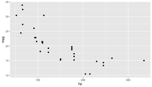
ggplot2
ggplot(data=mtcars,aes(x=hp,y=mpg,color=factor(cyl))) + geom_point()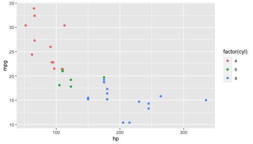
ggplot2
(g <- ggplot(data=mtcars,aes(x=hp,y=mpg,color=factor(cyl))) + geom_point() + geom_smooth(method="lm",se=FALSE) + geom_smooth(aes(x=hp,y=mpg,color="1"),color="black",method = "lm",se=FALSE) + labs(x="Some X-ax title",y="Some Y-ax title",title="Some title", color="Cyl",subtitle = "Some subtitle",caption="Source: My source") + scale_x_continuous(limits=c(0,400)) + scale_y_continuous(limits=c(0,50)) + theme_dark() + theme(legend.title = element_text(size=12)) + scale_color_manual(values=c("grey","green","pink"))) + facet_wrap(~factor(am))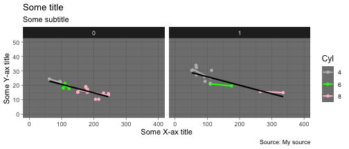
ggplot2
If you are interested in Data Viz, I highly recommend:
Data Visualization and Data Exploration using R
with Dr. Alicia Eads
Thursday, April 28, 1-4pm, SSMW 2022
Putting it together: two examples
The 2019 Canadian Election Study
https://dataverse.harvard.edu/dataset.xhtml?persistentId=doi:10.7910/DVN/8RHLG1
library(readstata13)df <- read.dta13("data/2019 Canadian Election Study - Phone Survey v1.0.dta")ces_2019_subset <- df %>% select(q2,q3,q4,q6,q9,q10,q11,q14,q15,q31,q32,weight_CES) %>% as_tibble()ces_2019_subset %>% glimpse()## Rows: 4,021## Columns: 12## $ q2 <int> 1963, 1973, 1994, 2000, 1984, 1939, 1999, 1995, 1963, 1970,…## $ q3 <fct> (1) Male, (1) Male, (1) Male, (1) Male, (1) Male, (1) Male,…## $ q4 <fct> (5) Quebec, (5) Quebec, (5) Quebec, (5) Quebec, (5) Quebec,…## $ q6 <fct> (3) Not very satisfied, (2) Fairly satisfied, (1) Very sati…## $ q9 <fct> (8), (10) Great deal of interest, (10) Great deal of intere…## $ q10 <fct> (1) Certain, (1) Certain, (1) Certain, (1) Certain, (1) Cer…## $ q11 <fct> "(-9) Don't know / Undecided", "(-9) Don't know / Undecided…## $ q14 <int> 60, 70, 70, 75, 10, 0, 50, 65, 50, 70, 15, 40, 50, 50, 90, …## $ q15 <int> 40, 55, 60, 40, 10, 30, 20, 25, 80, 10, 50, 25, 75, 0, -6, …## $ q31 <fct> (2) Worse, (3) About the same, (1) Better, (3) About the sa…## $ q32 <fct> (3) Not made much difference, (3) Not made much difference,…## $ weight_CES <dbl> 0.9019529, 0.9019529, 0.9019529, 1.2334642, 0.9019529, 0.90…ces_2019_subset <- ces_2019_subset %>% rename(q2_birthyear=q2,q3_gender=q3,q4_province=q4, q6_satisfied_democracy=q6,q9_interest_election=q9, q10_certain_vote=q10,q11_vote_intention=q11, q14_feeling_liberal_party=q14,q15_feeling_cons_party=q15, q31_ecnchange=q31,q32_policies_fed_gov_ecn=q32)ces_2019_subset <- ces_2019_subset %>% # Q14 and Q15 have negative values which should be NAs # See codebook mutate(q14_feeling_liberal_party=ifelse(q14_feeling_liberal_party<0, NA,q14_feeling_liberal_party), q15_feeling_cons_party=ifelse(q15_feeling_cons_party<0, NA,q15_feeling_cons_party))ces_2019_subset <- ces_2019_subset %>% mutate(q11_vote_intention=fct_recode(q11_vote_intention, "(4) Bloc Québécois (BQ, PQ, Bloc, Parti Québécois)"= "(4) Bloc Québécois (BQ, PQ, Bloc, Parti Québécois)"))ces_2019_subset %>% group_by(q3_gender) %>% summarise(avg_feeling_lib=mean(q14_feeling_liberal_party,na.rm=TRUE))## # A tibble: 3 × 2## q3_gender avg_feeling_lib## <fct> <dbl>## 1 (1) Male 44.3## 2 (2) Female 51.8## 3 (3) Other 40to_plot <- ces_2019_subset %>% group_by(q3_gender,q4_province) %>% summarise(avg_feeling_lib=mean(q14_feeling_liberal_party,na.rm=TRUE),.groups = 'drop')to_plot## # A tibble: 21 × 3## q3_gender q4_province avg_feeling_lib## <fct> <fct> <dbl>## 1 (1) Male (1) Newfoundland and Labrador 45.3## 2 (1) Male (2) Prince Edward Island 46.5## 3 (1) Male (3) Nova Scotia 49.4## 4 (1) Male (4) New Brunswick 47.8## 5 (1) Male (5) Quebec 49.2## 6 (1) Male (6) Ontario 50.3## 7 (1) Male (7) Manitoba 40.7## 8 (1) Male (8) Saskatchewan 32.1## 9 (1) Male (9) Alberta 24.7## 10 (1) Male (10) British Columbia 43.3## # … with 11 more rowsto_plot %>% filter(q3_gender!="(3) Other") %>% ggplot(aes(x=q3_gender,y=avg_feeling_lib,fill=q4_province)) + geom_bar(stat = "identity",position="dodge")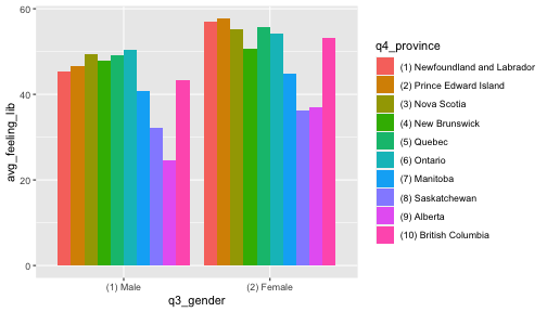
to_plot %>% filter(q3_gender!="(3) Other") %>% ggplot(aes(x=q3_gender,y=avg_feeling_lib,fill=q4_province)) + geom_bar(stat = "identity",position="dodge") + geom_text(aes(label=round(avg_feeling_lib)), position = position_dodge(width = .9),vjust=-0.25)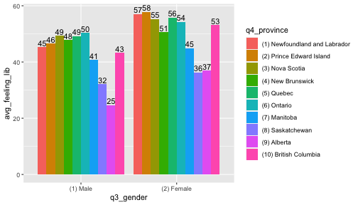
to_plot <- ces_2019_subset %>% mutate(q4_province_2=fct_recode(q4_province,"Atlantic"="(1) Newfoundland and Labrador", "Atlantic"="(2) Prince Edward Island", "Atlantic"="(3) Nova Scotia", "Atlantic"="(4) New Brunswick")) %>% group_by(q3_gender,q4_province_2) %>% summarise(avg_feeling_lib=mean(q14_feeling_liberal_party,na.rm=TRUE), .groups = 'drop')to_plot %>% filter(q3_gender!="(3) Other") %>% ggplot(aes(x=q3_gender,y=avg_feeling_lib,fill=q4_province_2)) + geom_bar(stat = "identity",position="dodge") + geom_text(aes(label=round(avg_feeling_lib)),position = position_dodge(width = .9),vjust=-0.25)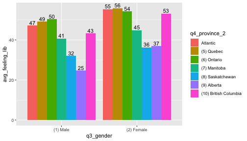
to_plot <- ces_2019_subset %>% mutate(q4_province_2=fct_recode(q4_province,"Atlantic"="(1) Newfoundland and Labrador", "Atlantic"="(2) Prince Edward Island", "Atlantic"="(3) Nova Scotia", "Atlantic"="(4) New Brunswick")) %>% group_by(q3_gender,q4_province_2) %>% summarise(avg_feeling_lib=weighted.mean(q14_feeling_liberal_party, weight_CES,na.rm=TRUE),.groups = 'drop')to_plot %>% filter(q3_gender!="(3) Other") %>% ggplot(aes(x=q3_gender,y=avg_feeling_lib, fill=q4_province_2)) + geom_bar(stat = "identity",position="dodge") + geom_text(aes(label=round(avg_feeling_lib)), position =position_dodge(width = .9),vjust=-0.25)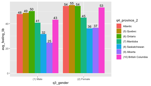
to_plot <- ces_2019_subset %>% mutate(q4_province_2=fct_recode(q4_province,"Atlantic"="(1) Newfoundland and Labrador", "Atlantic"="(2) Prince Edward Island", "Atlantic"="(3) Nova Scotia", "Atlantic"="(4) New Brunswick")) %>% group_by(q3_gender,q4_province_2) %>% summarise(avg_feeling_cons=weighted.mean(q15_feeling_cons_party,weight_CES,na.rm=TRUE), avg_feeling_lib=weighted.mean(q14_feeling_liberal_party,weight_CES,na.rm=TRUE),.groups = 'drop')to_plot %>% pivot_longer(c("avg_feeling_cons","avg_feeling_lib"),names_to = "party",values_to = "value") %>% filter(q3_gender!="(3) Other") %>% ggplot(aes(x=q3_gender,y=value,fill=party)) + geom_bar(stat = "identity",position="dodge") + geom_text(aes(label=round(value)),position = position_dodge(width = .9),vjust=-0.25) + facet_wrap(~q4_province_2) + scale_fill_manual(values=c("darkblue","red"))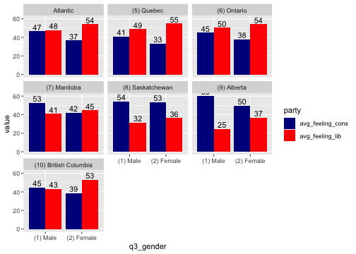
to_plot <- ces_2019_subset %>% filter(q31_ecnchange %in% c("(1) Better", "(2) Worse", "(3) About the same")) %>% mutate(q31_ecnchange=factor(q31_ecnchange,c("(2) Worse","(3) About the same","(1) Better"), labels=c("Worse","About the same","Better"))) %>% mutate(q4_province_2=fct_recode(q4_province,"Atlantic"="(1) Newfoundland and Labrador", "Atlantic"="(2) Prince Edward Island", "Atlantic"="(3) Nova Scotia", "Atlantic"="(4) New Brunswick")) %>% group_by(q3_gender,q4_province_2,q31_ecnchange) %>% summarise(sum_weightsQ31=sum(weight_CES),.groups = 'drop') %>% group_by(q3_gender,q4_province_2) %>% mutate(pc=sum_weightsQ31/sum(sum_weightsQ31))to_plot %>% ggplot(aes(x=q31_ecnchange,y=pc,fill=q3_gender)) + facet_wrap(~q4_province_2) + geom_bar(stat = "identity",position="dodge") + geom_text(aes(label=round(pc*100)),position = position_dodge(width = .9),vjust=-0.25) + labs(title="Feeling about the economy by gender and province")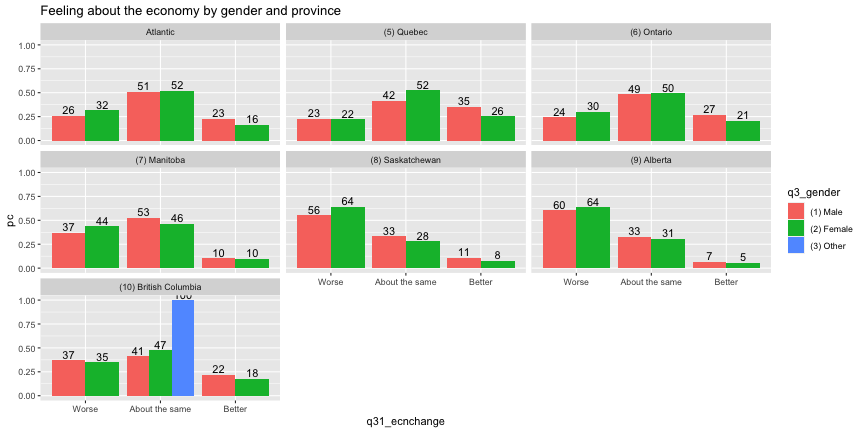
FeelingLibPartyi=B0+B1∗PoliciesFedGovEcni+B2∗birthyeari+B3∗genderi+ui
ces_2019_subset <- ces_2019_subset %>% filter(!(q31_ecnchange %in% c("(-9) Don't know", "(-8) Refused", "(-7) Skipped"))) %>% mutate(q31_ecnchange_numeric= as.numeric(factor(q31_ecnchange, c("(2) Worse","(3) Not made much difference","(1) Better"))))to_model <- ces_2019_subset %>% select(q14_feeling_liberal_party,q31_ecnchange_numeric, q2_birthyear,q3_gender,q4_province) %>% filter(complete.cases(.)) %>% mutate(age=2019-q2_birthyear)m <- lm(q14_feeling_liberal_party~q31_ecnchange_numeric+ age+q3_gender+q4_province,to_model)summary(m)## ## Call:## lm(formula = q14_feeling_liberal_party ~ q31_ecnchange_numeric + ## age + q3_gender + q4_province, data = to_model)## ## Residuals:## Min 1Q Median 3Q Max ## -71.498 -21.108 1.342 18.442 69.697 ## ## Coefficients:## Estimate Std. Error t value Pr(>|t|) ## (Intercept) 21.83572 3.28780 6.641 3.95e-11 ***## q31_ecnchange_numeric 16.39937 0.60896 26.930 < 2e-16 ***## age -0.14609 0.03379 -4.324 1.61e-05 ***## q3_gender(2) Female 7.47247 1.13553 6.581 5.91e-11 ***## q4_province(2) Prince Edward Island 0.87570 3.63661 0.241 0.80973 ## q4_province(3) Nova Scotia -4.54362 3.70761 -1.225 0.22053 ## q4_province(4) New Brunswick -2.47037 3.70780 -0.666 0.50532 ## q4_province(5) Quebec -0.58027 2.89823 -0.200 0.84133 ## q4_province(6) Ontario -0.75340 2.89516 -0.260 0.79471 ## q4_province(7) Manitoba -6.74018 3.46396 -1.946 0.05181 . ## q4_province(8) Saskatchewan -10.10906 3.25871 -3.102 0.00195 ** ## q4_province(9) Alberta -13.76282 3.21729 -4.278 1.97e-05 ***## q4_province(10) British Columbia -2.08257 2.86832 -0.726 0.46788 ## ---## Signif. codes: 0 '***' 0.001 '**' 0.01 '*' 0.05 '.' 0.1 ' ' 1## ## Residual standard error: 25.41 on 2082 degrees of freedom## Multiple R-squared: 0.3289, Adjusted R-squared: 0.325 ## F-statistic: 85.03 on 12 and 2082 DF, p-value: < 2.2e-16library(emmeans)emmeans(m,specs = "q31_ecnchange_numeric", at=list(q31_ecnchange_numeric=c(1,2,3)))## q31_ecnchange_numeric emmean SE df lower.CL upper.CL## 1 30.5 0.795 2082 29.0 32.1## 2 46.9 0.698 2082 45.5 48.3## 3 63.3 1.041 2082 61.3 65.3## ## Results are averaged over the levels of: q3_gender, q4_province ## Confidence level used: 0.95library(emmeans)emmeans(m,specs = "q31_ecnchange_numeric", at=list(q31_ecnchange_numeric=c(1,3))) %>% contrast( method = "pairwise", infer=TRUE)## contrast estimate SE df lower.CL upper.CL t.ratio p.value## 1 - 3 -32.8 1.22 2082 -35.2 -30.4 -26.930 <.0001## ## Results are averaged over the levels of: q3_gender, q4_province ## Confidence level used: 0.95to_model$prediction <- predict(m)myrmse <- round(sqrt(mean((to_model$q14_feeling_liberal_party- to_model$prediction)^2)),1)ggplot(to_model,aes(x=q14_feeling_liberal_party,y=prediction)) + geom_jitter() + labs(title=paste0("predictions and true values plotted: rmse=",myrmse))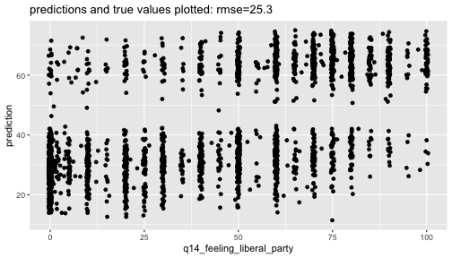
SCC cases
58 cases from the SCC in 2021. Can be accesses through link below. Can also be downloaded as a single zip.
library(tidyverse)library(textreadr)library(ldatuning)library(topicmodels)library(tidytext)# https://decisions.scc-csc.ca/scc-csc/scc-csc/en/2021/nav_date.dodownload.file("justinsavoie.com/data/2021.zip","~/Downloads/2021.zip")See https://www.tidytextmining.com/topicmodeling.html for more info on tidy text analysis.
folder_2021 <- "~/Downloads/2021"paths <- file.path(folder_2021,list.files(folder_2021))my_list <- list()for (k in 1:length(paths)){ doc <- textreadr::read_docx(paths[k]) citation <- str_replace(doc[2],"Citation: ","") start <- which(grepl("Present: ",doc))+3 end <- which(grepl("Cases Cited",doc))-1 if (length(start)==0 & length(end)==0){ next } doc_sub <- doc[start:end] df <- tibble(paragraph=paste0(doc_sub,collapse=" "),citation=citation) my_list[[k]] <- df %>% unnest_tokens(word, paragraph) %>% mutate(word=str_replace(word,"\\.","")) %>% filter(!grepl('[0-9]',word)) %>% filter(nchar(word)>4)}df_words <- bind_rows(my_list)df_words %>% group_by(citation,word) %>% summarise(n=n()) %>% group_by(citation) %>% mutate(pc=n/sum(n)) %>% arrange(citation,desc(pc)) %>% group_by(citation) %>% slice(1:5) %>% ungroup() %>% ggplot(aes(x=word,y=pc)) + geom_bar(stat="identity") + facet_wrap(~citation,scales = "free")dtm <- cast_dtm(df_words%>%group_by(citation,word)%>%summarise(n=n()), citation,word,n)modelLDA <- LDA(dtm,k=3)wtp <- tidy(modelLDA,matrix="beta")wtp %>% arrange(topic,desc(beta)) %>% group_by(topic) %>% slice(1:5) %>% mutate(term = reorder_within(term, beta, topic)) %>% ggplot(aes(y=term,fill=factor(topic),x=beta)) + geom_bar(stat = "identity",position = "dodge") + facet_wrap(~topic,ncol=1,scales = "free") + scale_y_reordered()Discussion of ideal number of topics https://cran.r-project.org/web/packages/ldatuning/vignettes/topics.html
result <- FindTopicsNumber( dtm, topics = seq(from = 2, to = 50, by = 1), metrics = c("Griffiths2004", "CaoJuan2009", "Arun2010", "Deveaud2014"), method = "Gibbs", verbose = TRUE)FindTopicsNumber_plot(result)modelLDA <- LDA(dtm,k=9)wtp <- tidy(modelLDA,matrix="beta")wtp %>% arrange(topic,desc(beta)) %>% group_by(topic) %>% slice(1:10) %>% mutate(term = reorder_within(term, beta, topic)) %>% ggplot(aes(y=term,x=beta)) + geom_bar(stat = "identity",position = "dodge") + facet_wrap(~topic,scales = "free") + scale_y_reordered()